Chatper 3. Storage and Retrieval
On the most fundamental level, a database needs to do two things:
- When you give it some data, it should store the data.
- When you ask it again later, it should give the data back to you.
Chapter 2 discussed data models and query languages, the format in which you (the application developer) give the database your data, and the mechanism by which you can ask for it again later.
This chapter is from the database's point of view: how we can store the data that we're given, and how we can find it again when we're asked for it.
As an application developer, you are probably not going to implement your own storage engine from scratch, but you do need to select a storage engine that is appropriate for your application. You need to care about how the database handles storage and retrieval internally.
In particular, there is a big difference between:
- Storage engines that are optimized for transactional workloads: see Transaction Processing or Analytics?
- Storage engines that are optimized for analytics: see Column-Oriented Storage
Data Structures That Power Your Database
Consider the world's simplest database, implemented as two Bash functions:
#!/bin/bash

db_set () {
    echo "$1,$2" >> database
}

db_get () {
    grep "^$1," database | sed -e "s/^$1,//" | tail -n 1
}
These two functions implement a key-value store:
- You can call
db_setkey value, which will store key and value in the database. The key and value can be anything you like, e.g., the value could be a JSON document. - You can then call
db_getkey, which looks up the most recent value associated with that particular key and returns it.
$ db_set 123456 '{"name":"London","attractions":["Big Ben","London Eye"]}'
$ db_set 42 '{"name":"San Francisco","attractions":["Golden Gate Bridge"]}'
$ db_get 42
{"name":"San Francisco","attractions":["Golden Gate Bridge"]}
The underlying storage format is very simple: a text file where each line contains a key-value pair, separated by a comma (roughly like a CSV file, ignoring escaping issues). Every call to db_set appends to the end of the file, so if you update a key several times, the old versions of the value are not overwritten, you need to look at the last occurrence of a key in a file to find the latest value (hence the tail -n 1 in db_get):
This db_set function actually has pretty good performance, because appending to a file is generally very efficient. Similarly to what db_set does, many databases internally use a log, which is an append-only data file. Real databases have more issues to deal with, for example:
- Concurrency control
- Reclaiming disk space so that the log doesn't grow forever
- Handling errors and partially written records
The word log is often used to refer to application logs, where an application outputs text that describes what's happening. In this book, log is used in the more general sense: an append-only sequence of records. It doesn't have to be human-readable; it might be binary and intended only for other programs to read.
On the other hand, the db_get function has terrible performance if you have a large number of records in your database. db_get has to scan the entire database file from beginning to end, looking for occurrences of the key. In algorithmic terms, the cost of a lookup is O(n).
In order to efficiently find the value for a particular key in the database, we need a different data structure: an index. The general idea behind index is to keep some additional metadata on the side, which acts as a signpost and helps you to locate the data you want. If you want to search the same data in several different ways, you may need several different indexes on different parts of the data.
An index is an additional structure that is derived from the primary data. Many databases allow you to add and remove indexes, and this doesn't affect the contents of the database; it only affects the performance of queries. Maintaining additional structures incurs overhead, especially on writes. For writes, it's hard to beat the performance of simply appending to a file, because that's the simplest possible write operation. Any kind of index usually slows down writes, because the index also needs to be updated every time data is written.
This is an important trade-off in storage systems: well-chosen indexes speed up read queries, but every index slows down writes. For this reason, databases don't usually index everything by default, but require you (the application developer or database administrator) to choose indexes manually, using your knowledge of the application's typical query patterns. You can then choose the indexes that give your application the greatest benefit, without introducing more overhead than necessary.
Hash Indexes
Although key-value data is not the only kind of data you can index, but it's very common, and it's a useful building block for more complex indexes.
Key-value stores are quite similar to the dictionary type that you can find in most programming languages, and which is usually implemented as a hash map (hash table).
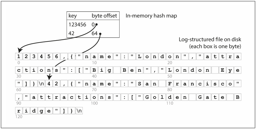
In the preceding example, our data storage consists only of appending to a file. Then the simplest possible indexing strategy is this: keep an in-memory hash map where every key is mapped to a byte offset in the data file, as illustrated in Figure 3-1.
- Whenever you append a new key-value pair to the file, you also update the hash map to reflect the offset of the data you just wrote (this works both for inserting new keys and for updating existing keys).
- When you want to look up a value, use the hash map to find the offset in the data file, seek to that location, and read the value.
This may sound simplistic, but it is a viable approach. In fact, this is essentially what Bitcask (the default storage engine in Riak) does:
- Bitcask offers high-performance reads and writes, subject to the requirement that all the keys fit in the available RAM, since the hash map is kept completely in memory.
- The values can use more space than there is available memory, since they can be loaded from disk with just one disk seek.
- If part of the data file is already in the filesystem cache, a read doesn't require any disk I/O at all.
A storage engine like Bitcask is well suited to situations where the value for each key is updated frequently. For example, the key is an URL of a cat video and the value might be the number of times it has been played. In this kind of workload, there are a lot of writes, but there are not too many distinct keys. Although you have a large number of writes per key, but it's feasible to keep all keys in memory.
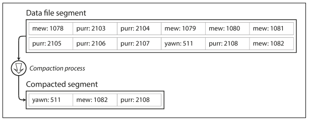
So far we only ever append to a file. How do we avoid eventually running out of disk space? A good solution is to break the log into segments of a certain size by closing a segment file when it reaches a certain size, and making subsequent writes to a new segment file. We can then perform compaction on these segments, as illustrated in Figure 3-2. Compaction means throwing away duplicate keys in the log, and keeping only the most recent update for each key.
Moreover, since compaction often makes segments much smaller (assuming that a key is overwritten several times on average within one segment), we can also merge several segments together at the same time as performing the compaction, as shown in Figure 3-3. Segments are never modified after they have been written, so the merged segment is written to a new file. The merging and compaction of frozen segments can be done in a background thread, and while it is going on, we can still continue to serve read and write requests as normal, using the old segment files. After the merging process is complete, we switch read requests to using the new merged segment instead of the old segments, and then the old segment files can simply be deleted.
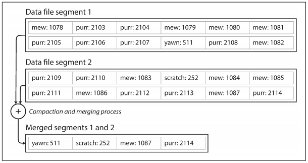
Each segment now has its own in-memory hash table, mapping keys to file offsets. In order to find the value for a key, we first check the most recent segment's hash map; if the key is not present we check the second-most-recent segment, and so on. The merging process keeps the number of segments small, so lookups don't need to check many hash maps.
Some of the issues that are important in a real implementation are:
- File format. CSV is not the best format for a log. It's faster and simpler to use a binary format that first encodes the length of a string in bytes, followed by the raw string (without need for escaping).
- Deleting records. If you want to delete a key and its associated value, you have to append a special deletion record to the data file (sometimes called a tombstone). When log segments are merged, the tombstone tells the merging process to discard any previous values for the deleted key.
- Crash recovery. If the database is restarted, the in-memory hash maps are lost. In principle, you can restore each segment's hash map by reading the entire segment file from beginning to end and noting the offset of the most recent value for every key as you go along. However, that might take a long time if the segment files are large, which would make server restarts painful. Bitcask speeds up recovery by storing a snapshot of each segment's hash map on disk, which can be loaded into memory more quickly.
- Partially written records. The database may crash at any time, including halfway through appending a record to the log. Bitcask files include checksums, allowing such corrupted parts of the log to be detected and ignored.
- Concurrency control. As writes are appended to the log in a strictly sequential order, a common implementation choice is to have only one writer thread. Data file segments are append-only and otherwise immutable, so they can be read concurrently by multiple threads.
An append-only log seems wasteful at first glance: why don't you update the file in place, overwriting the old value with the new value?
The append-only design turns out to be good for several reasons:
- Appending and segment merging are sequential write operations, which are generally much faster than random writes, especially on magnetic spinning-disk hard drives. To some extent sequential writes are also preferable on flash-based solid state drives (SSDs). See further discussions Comparing BTrees and LSM-Trees.
- Concurrency and crash recovery are much simpler if segment files are append-only or immutable. For example, you don't have to worry about the case where a crash happened while a value was being overwritten, leaving you with a file containing part of the old and part of the new value spliced together.
- Merging old segments avoids the problem of data files getting fragmented over time.
However, the hash table index also has limitations:
- The hash table must fit in memory, so if you have a very large number of keys, you're out of luck. In principle, you could maintain a hash map on disk, but unfortunately it is difficult to make an on-disk hash map perform well. It requires a lot of random access I/O, it is expensive to grow when it becomes full, and hash collisions require fiddly logic.
- Range queries are not efficient. For example, you cannot easily scan over all keys between
kitty00000andkitty99999. You'd have to look up each key individually in the hash maps.
The indexing structure in the next section doesn't have those limitations.
SSTables and LSM-Trees
In Figure 3-3, each log-structured storage segment is a sequence of key-value pairs. These pairs appear in the order that they were written, and values later in the log take precedence over values for the same key earlier in the log. Apart from that, the order of key-value pairs in the file does not matter.
Now we can make a simple change to the format of our segment files: we require that the sequence of key-value pairs is sorted by key. At first glance, that requirement seems to break our ability to use sequential writes (to be discussed later).
We call this format Sorted String Table, or SSTable for short. We also require that each key only appears once within each merged segment file (the compaction process already ensures that).
SSTables have several big advantages over log segments with hash indexes:
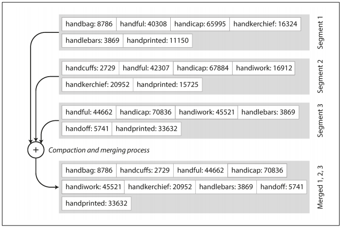
- Merging segments is simple and efficient, even if the files are bigger than the available memory. The approach is like the one used in the mergesort algorithm and is illustrated in Figure 3-4 (above): read the input files side by side, for the first key in each file, copy the lowest key (according to the sort order) to the output file, and repeat. This produces a new merged segment file, also sorted by key. When multiple segments contain the same key, keep the value from the most recent segment and discard the values in older segments. [p77]
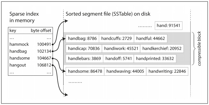
- In order to find a particular key in the file, you no longer need to keep an index of all the keys in memory. See Figure 3-5 (below) for an example: you're looking for the key
handiwork, but you don't know the exact offset of that key in the segment file. However, you do know the offsets for the keyshandbagandhandsome, and because of the sorting you know thathandiworkmust appear between those two. This means you can jump to the offset forhandbagand scan from there until you findhandiwork(or not, if the key is not present in the file).- You still need an in-memory index to tell you the offsets for some of the keys, but it can be sparse: one key for every few kilobytes of segment file is sufficient, because a few kilobytes can be scanned very quickly.
- If all keys and values had a fixed size, you could use binary search on a segment file and avoid the in-memory index entirely. However, they are usually variable-length in practice, which makes it difficult to tell where one record ends and the next one starts if you don't have an index.
- Since read requests need to scan over several key-value pairs in the requested range anyway, it is possible to group those records into a block and compress it before writing it to disk (indicated by the shaded area in Figure 3-5). Each entry of the sparse in-memory index then points at the start of a compressed block. Besides saving disk space, compression also reduces the I/O bandwidth use.
Constructing and maintaining SSTables
How do you get your data to be sorted by key in the first place? Incoming writes can occur in any order.
Maintaining a sorted structure on disk is possible (see B-Trees in the upcoming section), but maintaining it in memory is much easier. With a plenty of well-known tree data structures you can use, such as red-black trees or AVL trees, you can insert keys in any order and read them back in sorted order.
We can now make our storage engine work as follows:
- When a write comes in, add it to an in-memory balanced tree data structure (for example, a red-black tree). This in-memory tree is sometimes called a memtable.
- When the memtable gets bigger than some threshold (typically a few megabytes) write it out to disk as an SSTable file. This can be done efficiently because the tree already maintains the key-value pairs sorted by key. The new SSTable file becomes the most recent segment of the database. While the SSTable is being written out to disk, writes can continue to a new memtable instance.
- In order to serve a read request, first try to find the key in the memtable, then in the most recent on-disk segment, then in the next-older segment, etc.
- From time to time, run a merging and compaction process in the background to combine segment files and to discard overwritten or deleted values.
This works very well except for one problem: if the database crashes, the most recent writes (which are in the memtable but not yet written out to disk) are lost. In order to avoid that problem, we can keep a separate log on disk to which every write is immediately appended, just like in the previous section. That log is not in sorted order, but that doesn't matter, because its only purpose is to restore the memtable after a crash. Every time the memtable is written out to an SSTable, the corresponding log can be discarded.
Making an LSM-tree out of SSTables
The algorithm described here is essentially what is used in LevelDB and RocksDB, key-value storage engine libraries that are designed to be embedded into other applications. Among other things, LevelDB can be used in Riak as an alternative to Bitcask. Similar storage engines are used in Cassandra and HBase, both of which were inspired by Google's Bigtable paper.
Originally this indexing structure was described by Patrick O'Neil et al. under the name Log-Structured Merge-Tree (or LSM-Tree), building on earlier work on log-structured filesystems. Storage engines that are based on this principle of merging and compacting sorted files are often called LSM storage engines.
Lucene, an indexing engine for full-text search used by Elasticsearch and Solr, uses a similar method for storing its term dictionary. A full-text index is much more complex than a key-value index but is based on a similar idea: given a word in a search query, find all the documents (web pages, product descriptions, etc.) that mention the word. This is implemented with a key-value structure where the key is a word (a term) and the value is the list of IDs of all the documents that contain the word (the postings list). In Lucene, this mapping from term to postings list is kept in SSTable-like sorted files, which are merged in the background as needed.
Performance optimizations
As always, a lot of detail goes into making a storage engine perform well in practice. For example, the LSM-tree algorithm can be slow when looking up keys that do not exist in the database: you have to check the memtable, then the segments all the way back to the oldest before you can be sure that the key does not exist. In order to optimize this kind of access, storage engines often use additional Bloom filters. (A Bloom filter is a memory-efficient data structure for approximating the contents of a set. It can tell you if a key does not appear in the database, and thus saves many unnecessary disk reads for nonexistent keys.)
There are also different strategies to determine the order and timing of how SSTables are compacted and merged. The most common options are size-tiered and leveled compaction. LevelDB and RocksDB use leveled compaction (hence the name of LevelDB), HBase uses size-tiered, and Cassandra supports both.
- In size-tiered compaction, newer and smaller SSTables are successively merged into older and larger SSTables. (See DS210 Size Tiered Compaction)
- In leveled compaction, the key range is split up into smaller SSTables and older data is moved into separate "levels", which allows the compaction to proceed more incrementally and use less disk space. (See DS210 Leveled Compaction)
Even though there are many subtleties, the basic idea of LSM-trees is keeping a cascade of SSTables that are merged in the background, which is simple and effective. Even when the dataset is much bigger than the available memory it continues to work well. Since data is stored in sorted order, you can efficiently perform range queries (scanning all keys above some minimum and up to some maximum), and because the disk writes are sequential the LSM-tree can support remarkably high write throughput.
B-Trees
Though gaining acceptance, the log-structured indexes are not the most common type of index. The most widely used indexing structure is quite different: the B-tree.
Introduced in 1970 and called "ubiquitous" less than 10 years later, B-trees remain the standard index implementation in almost all relational databases, and also used by many non-relational databases.
Like SSTables, B-trees keep key-value pairs sorted by key, which allows efficient key-value lookups and range queries. But that's where the similarity ends: B-trees have a very different design philosophy.
The log-structured indexes break the database down into variable-size segments, typically several megabytes or more in size, and always write a segment sequentially. By contrast, B-trees break the database down into fixed-size blocks or pages, traditionally 4 KB in size (sometimes bigger), and read or write one page at a time. This design corresponds more closely to the underlying hardware, as disks are also arranged in fixed-size blocks.
Each page can be identified using an address or location, which allows one page to refer to another (similar to a pointer, but on disk instead of in memory). We can use these page references to construct a tree of pages, as illustrated in Figure 3-6 (below).
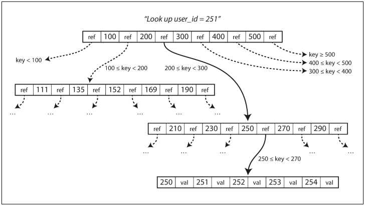
- One page is designated as the root of the B-tree, which is where you starts your lookup.
- The page contains several keys and references to child pages.
- Each child is responsible for a continuous range of keys, and the keys between the references indicate where the boundaries between those ranges lie.
In the Figure 3-6 example (above), we are looking for the key 251, so we know that we need to follow the page reference between the boundaries 200 and 300. That takes us to a similar-looking page that further breaks down the 200–300 range into subranges. Eventually we get down to a page containing individual keys (a leaf page), which either contains the value for each key inline or contains references to the pages where the values can be found.
The number of references to child pages in one page of the B-tree is called the branching factor. For example, in Figure 3-6 the branching factor is six. In practice, the branching factor depends on the amount of space required to store the page references and the range boundaries, but typically it is several hundred.
- If you want to update the value for an existing key in a B-tree, you search for the leaf page containing that key, change the value in that page, and write the page back to disk (any references to that page remain valid).
- If you want to add a new key, you need to find the page whose range encompasses the new key and add it to that page. If there isn't enough free space in the page to accommodate the new key, it is split into two half-full pages, and the parent page is updated to account for the new subdivision of key ranges. See Figure 3-7 (below).
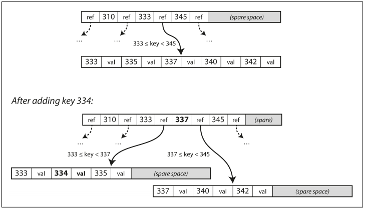
This algorithm ensures that the tree remains balanced: a B-tree with n keys always has a depth of O(log n). Most databases can fit into a B-tree with a depth of three or four levels, so you don't need to follow many page references to find the page. (A four-level tree of 4 KB pages with a branching factor of 500 can store up to 256 TB.)
Making B-trees reliable
The underlying write operation of a B-tree is to overwrite a page on disk with new data. It is assumed that the overwrite does not change the location of the page: all references to that page remain intact when the page is overwritten. This is in contrast to log-structured indexes such as LSM-trees, which only append to files (and eventually delete obsolete files) but never modify files in place.
You can think of overwriting a page on disk as an actual hardware operation:
- On a magnetic hard drive, this means moving the disk head to the right place, waiting for the right position on the spinning platter to come around, and then overwriting the appropriate sector with new data.
- On SSDs, what happens is somewhat more complicated, due to the fact that an SSD must erase and rewrite fairly large blocks of a storage chip at a time.
Moreover, some operations require several different pages to be overwritten. For example, if you split a page because an insertion caused it to be overfull, you need to write the two pages that were split, and also overwrite their parent page to update the references to the two child pages. This is a dangerous operation, because if the database crashes after only some of the pages have been written, you end up with a corrupted index (e.g., there may be an orphan page that is not a child of any parent).
In order to make the database resilient to crashes, it is common for B-tree implementations to include an additional data structure on disk: a write-ahead log (WAL, also known as a redo log). This is an append-only file to which every B-tree modification must be written before it can be applied to the pages of the tree itself. When the database comes back up after a crash, this log is used to restore the B-tree back to a consistent state.
Concurrency control is required if multiple threads are going to access the B-tree at the same time, otherwise a thread may see the tree in an inconsistent state. This is typically done by protecting the tree's data structures with latches (lightweight locks). (In this regard, log-structured approaches are simpler in this regard, because they do all the merging in the background without interfering with incoming queries and atomically swap old segments for new segments from time to time.)
B-tree optimizations
Many optimizations for B-trees have been developed over the years, such as:
- Instead of overwriting pages and maintaining a write-ahead log for crash recovery, some databases (like LMDB) use a copy-on-write scheme. A modified page is written to a different location, and a new version of the parent pages in the tree is created, pointing at the new location. This approach is also useful for concurrency control (see Snapshot Isolation and Repeatable Read in Chapter 7).
- We can save space in pages by not storing the entire key, but abbreviating it. Especially in pages on the interior of the tree, keys only need to provide enough information to act as boundaries between key ranges. Packing more keys into a page allows the tree to have a higher branching factor, and thus fewer levels. (This variant is sometimes known as a B+ tree, although the optimization is so common that it often isn't distinguished from other B-tree variants.)
- In general, pages can be positioned anywhere on disk; there is nothing requiring pages with nearby key ranges to be nearby on disk. If a query needs to scan over a large part of the key range in sorted order, that page-by-page layout can be inefficient, because a disk seek may be required for every page that is read. Many B-tree implementations therefore try to lay out the tree so that leaf pages appear in sequential order on disk. However, it's difficult to maintain that order as the tree grows.
- By contrast, since LSM-trees rewrite large segments of the storage in one go during merging, it's easier for them to keep sequential keys close to each other on disk.
- Additional pointers have been added to the tree. For example, each leaf page may have references to its sibling pages to the left and right, which allows scanning keys in order without jumping back to parent pages.
- B-tree variants such as fractal trees borrow some log-structured ideas to reduce disk seeks.
Comparing B-Trees and LSM-Trees
B-tree implementations are generally more mature, but LSM-trees are also interesting due to their performance characteristics.
As a rule of thumb, LSM-trees are typically faster for writes, whereas B-trees are thought to be faster for reads. Reads are typically slower on LSM-trees because they have to check several different data structures and SSTables at different stages of compaction.
However, benchmarks are often inconclusive and sensitive to details of the workload. You need to test systems with your particular workload in order to make a valid comparison.
Advantages of LSM-trees
A B-tree index must write every piece of data at least twice: once to the write-ahead log, and once to the tree page itself (and again as pages are split). There is also overhead from having to write an entire page at a time, even if only a few bytes in that page changed. Some storage engines even overwrite the same page twice in order to avoid ending up with a partially updated page in the event of a power failure (such as InnoDB).
Log-structured indexes also rewrite data multiple times due to repeated compaction and merging of SSTables. One write to the database resulting in multiple writes to the disk over the course of the database's lifetime. This effect is known as write amplification. It is of particular concern on SSDs, which can only overwrite blocks a limited number of times before wearing out (see also wear leveling).
In write-heavy applications, the performance bottleneck might be the rate at which the database can write to disk. In this case, write amplification has a direct performance cost: the more that a storage engine writes to disk, the fewer writes per second it can handle within the available disk bandwidth.
Moreover, LSM-trees are typically able to sustain higher write throughput than B-trees, partly because:
- They sometimes have lower write amplification (although this depends on the storage engine configuration and workload),
- They sequentially write compact SSTable files rather than having to overwrite several pages in the tree.
This difference is particularly important on magnetic hard drives, where sequential writes are much faster than random writes.
LSM-trees can be compressed better, and thus often produce smaller files on disk than B-trees. B-tree storage engines leave some disk space unused due to fragmentation: when a page is split or when a row cannot fit into an existing page, some space in a page remains unused. Since LSM-trees are not page-oriented and periodically rewrite SSTables to remove fragmentation, they have lower storage overheads, especially when using leveled compaction
On many SSDs, the firmware internally uses a log-structured algorithm to turn random writes into sequential writes on the underlying storage chips, so the impact of the storage engine's write pattern is less pronounced. However, lower write amplification and reduced fragmentation are still advantageous on SSDs: representing data more compactly allows more read and write requests within the available I/O bandwidth.
Downsides of LSM-trees
A downside of log-structured storage is that the compaction process can sometimes interfere with the performance of ongoing reads and writes. Since disks have limited resources, so it can easily happen that a request needs to wait while the disk finishes an expensive compaction operation. The impact on throughput and average response time is usually small, but at higher percentiles the response time of queries to log-structured storage engines can sometimes be quite high, and B-trees can be more predictable.
At high write throughput, the disk's finite write bandwidth needs to be shared between the initial write (logging and flushing a memtable to disk) and the compaction threads running in the background. The bigger the database gets, the more disk bandwidth is required for compaction.
If write throughput is high and compaction is not configured carefully, it can happen that compaction cannot keep up with the rate of incoming writes. In this case, the number of unmerged segments on disk keeps growing until you run out of disk space, and reads also slow down because they need to check more segment files. Typically, SSTable-based storage engines do not throttle the rate of incoming writes, even if compaction cannot keep up, so you need explicit monitoring to detect this situation.
Advantages of B-trees *
An advantage of B-trees is that each key exists in exactly one place in the index, whereas a log-structured storage engine may have multiple copies of the same key in different segments. This aspect makes B-trees attractive in databases that want to offer strong transactional semantics: in many relational databases, transaction isolation is implemented using locks on ranges of keys, and in a B-tree index, those locks can be directly attached to the tree. See more details in Chapter 7.
B-trees are very ingrained in the architecture of databases and provide consistently good performance for many workloads, so it's unlikely that they will go away anytime soon. In new datastores, log-structured indexes are becoming increasingly popular. There is no quick and easy rule for determining which type of storage engine is better for your use case, so it is worth testing empirically.
Other Indexing Structures
So far we have only discussed key-value indexes, which are like a primary key index in the relational model. A primary key uniquely identifies one row in a relational table, or one document in a document database, or one vertex in a graph database. Other records in the database can refer to that row/document/vertex by its primary key (or ID), and the index is used to resolve such references.
It is also very common to have secondary indexes. In relational databases, you can create several secondary indexes on the same table using the CREATE INDEX command, and they are often crucial for performing joins efficiently. For example, in Figure 2-1 in Chapter 2 you would most likely have a secondary index on the user_id columns so that you can find all the rows belonging to the same user in each of the tables.
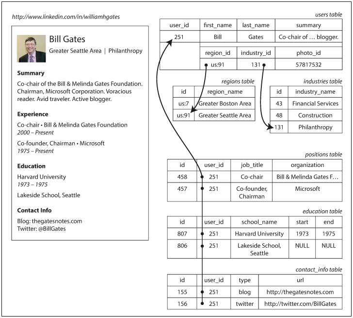
A secondary index can easily be constructed from a key-value index. The main difference is that the indexed values in a secondary index are not necessarily unique; that is, there might be many rows (documents, vertices) under the same index entry. This can be solved in two ways: either by making each value in the index a list of matching row identifiers (like a postings list in a full-text index) or by making each entry unique by appending a row identifier to it. Either way, both B-trees and log-structured indexes can be used as secondary indexes.
Storing values within the index
The key in an index is the thing that queries search for, but the value can be one of two things: it could be the actual row (document, vertex), or it could be a reference to the row. In the latter case, the place where rows are stored is known as a heap file, and it stores data in no particular order (it may be append-only, or it may keep track of deleted rows in order to overwrite them with new data later). The heap file approach is common because it avoids duplicating data when multiple secondary indexes are present: each index just references a location in the heap file, and the actual data is kept in one place.
When updating a value without changing the key, the heap file approach can be quite efficient: the record can be overwritten in place, provided that the new value is not larger than the old value. The situation is more complicated if the new value is larger, as it probably needs to be moved to a new location in the heap where there is enough space. In that case, either all indexes need to be updated to point at the new heap location of the record, or a forwarding pointer is left behind in the old heap location.
In some situations, the extra hop from the index to the heap file is too much of a performance penalty for reads, so it can be desirable to store the indexed row directly within an index. This is known as a clustered index. For example, in MySQL's InnoDB storage engine, the primary key of a table is always a clustered index, and secondary indexes refer to the primary key (rather than a heap file location). In SQL Server, you can specify one clustered index per table.
A compromise between a clustered index (storing all row data within the index) and a nonclustered index (storing only references to the data within the index) is known as a covering index or index with included columns, which stores some of a table's columns within the index. This allows some queries to be answered by using the index alone (in which case, the index is said to cover the query).
As with any kind of duplication of data, clustered and covering indexes can speed up reads, but they require additional storage and can add overhead on writes. Databases also need to go to additional effort to enforce transactional guarantees, because applications should not see inconsistencies due to the duplication.